Matrix multiplication is one of the concepts where reading the formula is easy, but developing intuition takes more time. Since it is such a common concept in linear algebra, in this post we try to develop a better intuition for it.

Matrix multiplication is formally defined as follows - if $A$ is a matrix of size $m \times n$ and $B$ is a matrix of size $n \times p$, then $C = A \cdot B$ is a matrix of size $m \times p$, where its cells are given by

\[C_{ij}=\sum_{k=1}^{n} A_{ik} \cdot B_{kj}\]

In other words, the cell at row $i$ and column $j$ in $C$ is calculated by summing the products of each item in the $i$-th row of $A$ and the $j$-th column of $B$.

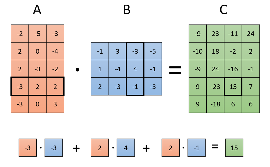
Stopping the explanation at this point, however, is doing matrix multiplication an injustice - this technical definition does not show the situations in which matrix multiplications might arise, or help understand how its output is affected by its input. To make things worse, the same concept has multiple possible interpretations each suitable to a different situation, and having in mind an interpretation unsuitable for a given situation might only make things more confusing.

The goal of this post, therefore, is to outline some common interpretations of matrix multiplication, propose how to best mentally visualize them, and help identify when each of them might be useful.

A key to having a good intuition in mind is to be very clear and explicit about what the input and output represent. We therefore start with describing the various options to think about them.

The Data

Vectors

The most basic building block of linear algebra is a vector, which is just an array of numbers:

This bare-bones representation is mainly useful when each cell describes a completely different property in a different scale, which just happen to be grouped in an arbitrary ordering.

For example, if the vector represents the attributes of a house, the first cell might contain the number of houses, the second its size in some unit, and the third the number of balconies.

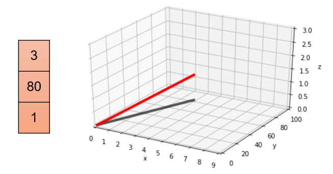
Sometimes, however, we prefer to think of these numbers as coordinates of a space. While this is always possible, it is mainly helpful when all cells contain numbers with similar meaning and scale (otherwise distances and angles don’t tell us much). It is then helpful to imagine the vector as a point in space, or an arrow from the origin to that point:

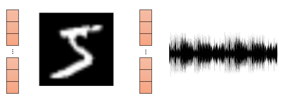
Lastly, sometimes our vectors represent objects in some domain such as an image or an audiowave. While also made of numbers, they may have domain-specific interpretation, e.g. making all numbers composing an image smaller makes the image darker.

The appropriate visualization for a vector generally depends on the context in which it is going to be used. For that, let us introduce a way to group vectors together and to apply transformations to them.

Matrices

Another important building block is the matrix, which is a two-dimensional array of numbers, also known as a table:

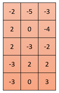
While all matrices are made up of such numbers, sometimes the numbers come with an additional meaning. The most simple example is a matrix that is formed by grouping vectors, either as rows or as columns:

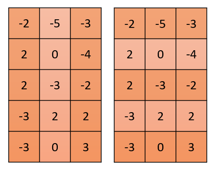
Beside storing data, every matrix can also be used as a transformation which takes a vector as an input and returns another vector as its output. Instead of saying we apply the matrix to a vector, we say we multiply the matrix with the vector.

While we will get to the way such a transformation works later in this post, a key idea is that when a matrix is interpreted as a transformation then what we visualize, instead of the content of the matrix, is usually its effect on vectors.

Now that we understand how to think about the data, let’s see how to think about transformations we can apply to it.

Multiplications

To build up to multiplying a matrix by a matrix, we start with multiplying a vector by a vector.

Vector-vector multiplication

Multiplying a vector $v$ with a vector $u$ gives a single number, a scalar, that is calculated with the formula

\[\sum_{i=1}^{n} v_{i} \cdot u_{i}\]

which we have seen appearing for each cell in the output matrix in the introduction. This product is also called a dot product or scalar product.

Based on what the vectors represent, we can give this operation different interpretations:

1. When one of the vectors is a set of coefficients, the multiplication uses these coefficients to form a weighted combination of the cells of the other vectors.

   

   In the house prices setting, if the $i$-th cell of $v$ contains some attribute of the house and the corresponding cell of $u$ contains the money we can expect for one unit of this attribute, then $v \cdot u$ gives us the total cost of the house.

2. When both vectors are interpreted as points in space, there is an additional formula to calculate the product based on geometric properties:

   \[v \cdot u = \|v\| \cdot \|u\| \cdot \cos(\theta)\]

   Where $|v|$ is the length of $v$, $|u|$ is the length of $u$ and $ \theta $ is the angle between them. Notice that the right-hand side does not contain vectors, only scalars.

   This is mainly interesting when one of the length of $u$ is 1, because then the product is the projection of $v$ onto $u$:

   

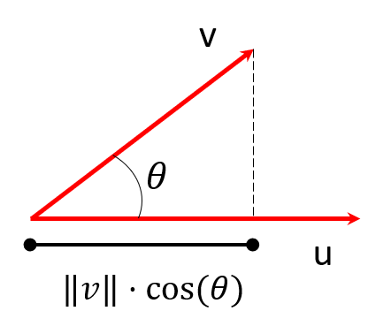
   When both lengths are constant (e.g. they are 1) then a higher result corresponds to the angle $\theta$ being more acute. Then the product measures “how similar are $u$ and $v$”, as an easier way to say “between $-1$ and $1$, how much are $u$ and $v$ pointing in the same direction” (with $1$ noting same direction, $-1$ being opposite directions, and $0$ being orthogonal).

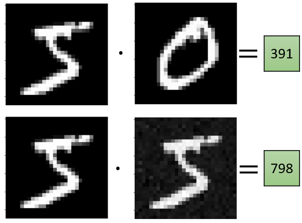
3. When both vectors represent an object of the same type (for example, an image) we still interpret their product as similarity or correlation, without thinking about angles.

   

Matrix-vector multiplication

The interpretation for a product of the form $u = A \cdot v$ highly depends on what $A$ and $v$ represent.

1. When $A$ is a list of row vectors, the resulting vector is a list of scalar results, which are many independent vector-vector multiplications. In the house prices example - this is a calculation of the total price of multiple houses, simultaneously.

2. When $A$ is a list of column vectors, and the vector is a list of coefficients, the multiplication creates a combination of the columns of $A$ into a single column using $v$:

   

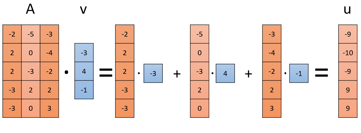
   For example, the columns of $A$ could be ingredients of various fruits, combined to form a vector describing the ingredients of a salad.

3. When $A$ is a transformation and $v$ is a point or object to be transformed by $A$, $u$ is the $v$ after being transformed.

   If $v$ is a point and $A$ is a geometric operation such as a rotation or scaling, then $u$ is the transformed point:

   

   If $v$ is a higher-level object such as an image, and $A$ is a transformation such as blurring, then $u$ is the transformed object:

   

It is easy to get confused by 2 and 3. In 2, $v$ transforms the data in $A$, while in 3 the transformation $A$ acts on the data $v$.

Matrix-matrix multiplication

In a matrix-matrix multiplication of the form $C = A \cdot B$, the first step is to figure out what $B$ represents.

1. The simplest and most common case is when $B$ is a list of column vectors. In this case, the multiplication can be broken down to a list of independent multiplications from the previous section, which we interpret using the guidelines from before, based on what $A$ represents. Since multiple results are returned, what was previously a scalar becomes a vector and vectors become matrices.

   a. When $A$ is a transformation, then the resulting $C$ is a list of the vectors in $B$ after having been transformed by $A$.

   b. If $A$ is a list of row vectors, the result is a list of lists, i.e. a table, where the cell at index $i,j$ is the dot product of row $i$ of $A$ with column $j$ of $B$, as in the first visualization we’ve seen. This usually describes a case where $A$ and $B$ store two lists of the same size containing objects that can interact - for example, houses and different house pricings, user preferences and items, words and documents.

   c. When $A$ is a list of column vectors, then the resulting $C$ is a list of column vectors, each formed as a different weighted combination of the columns of $A$ - column $j$ of $C$ is a weighted combination of the columns of $A$ with the coefficients in column $j$ of $B$.

2. When $A$ and $B$ are both transformations, then $C$ too is a transformation that is achieved by applying $C$ and then $A$, since:

   \[C \cdot v = (A \cdot B) \cdot v = A \cdot (B \cdot v)\]

   For example if $A$ rotates vectors and $B$ shrinks them in one direction, $C$ will first shrink them and then rotate them.

Conclusion

Hopefully, by now it is clear that the same concept can be visualized in multiple ways, and when these might be useful.

While this list of visualizations might seem long, it is important to emphasize that some of these situations are much more common than others. Some other, less common interpretations have been left out (e.g. operations on rows, block matrices, sum of projections) and might be dealt with in a future post.

The key takeaway is that being clear and explicit about what the matrices represent enables choosing the most helpful mental visualization.